Building a $34 ESP32 Parts Counter Using Blob Detection

If you've ever spent time counting small electronic components, hardware, or any tiny parts, you know the struggle: it's tedious, error-prone, and surprisingly time-consuming. I decided to solve this problem with a self-contained parts counter built around an ESP32 microcontroller for just $34.
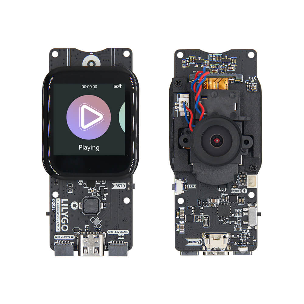
I used the LilyGo T-Camera Plus S3. But you could use any just about any ESP32 with a camera.
https://lilygo.cc/en-us/products/t-camera-plus-s3
The Hardware: ESP32 Camera Module
For this project, I used an ESP32 development board with an integrated camera module and display. While I originally prototyped with a LilyGO T-Camera Plus (which combines an ESP32, camera, and screen in one compact package), these aren't always readily available. The good news is that the code should work with most ESP32-CAM boards paired with a small display.
Why ESP32?
The ESP32 is perfect for this application because:
- Sufficient processing power for real-time image processing
- Built-in camera interface for OV2640 and similar modules
- Low cost - the entire BOM comes in around $34
- Self-contained - no laptop or external computer needed
- Low power consumption - can run on battery if needed
Bill of Materials
- ESP32 camera board (ESP32-CAM or similar): ~$10-15
- Small TFT display (if not integrated): ~$8-12
- 3D printed backlight tray with LED strips: ~$5
- 3D printed camera mount: ~$2
- Misc wiring and power supply: ~$5
Total: approximately $34
The Algorithm: Blob Detection
Rather than jumping straight to machine learning (which would be overkill for this application), I went with a classic computer vision technique called blob detection using connected-component labeling.
Why Not Machine Learning?
Before the comments fill up with "you should use a neural network," let me explain why I didn't:
- Training overhead - Every new part type requires collecting training images and retraining
- Processing power - Neural networks need significantly more compute resources
- Complexity - A CNN would be massive overkill for counting identical objects
- Perfect use case for classical CV - When objects are similar and lighting is controlled, blob detection is fast, reliable, and simple
How Blob Detection Works
Here is a simulator that let's you try it for yourself...

https://qwerte.com/BlobCounter.html
Step 1: Binary Conversion
The captured image is converted to pure binary (not grayscale - actual 1-bit black and white). Objects become white pixels, and the background becomes black pixels. This is controlled by the Threshold parameter.
Step 2: Scanning and Flood-Fill
The algorithm scans the image line-by-line, pixel-by-pixel. When it encounters a white pixel that hasn't been processed yet:
- It marks that pixel as part of a new blob
- It flood-fills all connected white pixels, expanding outward
- Each connected region becomes one "blob"

Step 3: Size Filtering
Once all blobs are identified, each one is measured by its pixel count. The algorithm applies two filters:
- Minimum Blob Size - Rejects small noise, dust, and artifacts
- Maximum Blob Size - Rejects anything larger than expected (merged parts or debris)
Step 4: Final Count
All valid blobs (within the min/max range) are counted and displayed on the screen.
The Three Tuning Parameters
Getting accurate counts requires adjusting three key parameters for your specific parts and lighting:
1. Threshold (0-255) This sets the brightness level that separates objects from background. Too low and parts get lost in the background. Too high and shadows or reflections become false positives.
2. Minimum Blob Size (pixels) Filters out dust, scratches, and image noise. Set this just below the smallest valid part size.
3. Maximum Blob Size (pixels) Prevents merged parts or large debris from being counted. Set this just above the largest valid part size.
The Lighting Challenge
Good software is useless without good input data. Getting clean, consistent images turned out to be the hardest part of this project.

Attempt #1: Single Point Light
My first try used a simple desk lamp at an angle. Result: Failure.
The harsh shadows completely distorted the part silhouettes. Some parts appeared merged while others had shadows that made them look like multiple objects.
Attempt #2: Ring Light
Next, I tried a LED ring light mounted around the camera. Result: Also failure.
While it eliminated harsh shadows, it created multiple problems:
- Specular highlights on shiny parts broke up the silhouettes
- Parts touching each other cast shadows between them, causing the algorithm to merge them into one blob
- Inconsistent lighting across the counting area
Attempt #3: Backlighting (The Winner!)
Backlighting solved everything. By placing a diffused light source under the parts, I got:
- Perfect silhouettes with crisp edges
- No shadows between parts
- No specular highlights
- Consistent lighting across the entire field of view
Even when parts slightly overlap, enough light gets through to keep them separated in the binary image.
The 3D Printed Counting Tray

To implement backlighting, I designed a custom counting tray in Fusion 360:
Design Features:
- LED strip channel - Holds a strip of white LEDs around the perimeter
- Diffuser platform - Translucent white surface (I used 3mm white acrylic, but you could print a thin layer)
- Raised edges - Keeps parts contained in the counting area
- Mounting posts - Attaches the camera mount at a fixed height
The tray measures approximately 150mm x 150mm, giving a decent counting area while keeping the camera close enough for good resolution.
Camera Mount
The camera mount attaches to the tray and holds the ESP32 at a fixed distance and angle. This consistency is crucial - if the camera moves or tilts, the region of interest and scale calibration become invalid.
Key features:
- Fixed height - Maintains consistent field of view
- Angled bracket - Camera points straight down at 90°
- Cable management - Routes the USB power cable cleanly
Software Implementation
The code is structured into several key components:
Image Capture and Processing
// Capture image from camera
camera_fb_t *fb = esp_camera_fb_get();

// Convert to binary using threshold
for (int i = 0; i < fb->len; i++) {
    binaryImage[i] = (fb->buf[i] > threshold) ? 255 : 0;
}

esp_camera_fb_return(fb);
Blob Detection via Connected-Component Labeling
The heart of the algorithm uses a flood-fill approach:
int blobCount = 0;
for (int y = roi.y; y < roi.y + roi.height; y++) {
    for (int x = roi.x; x < roi.x + roi.width; x++) {
        if (isWhitePixel(x, y) && !isLabeled(x, y)) {
            int blobSize = floodFill(x, y, blobCount);

            if (blobSize >= minBlobSize && blobSize <= maxBlobSize) {
                blobCount++;
            }
        }
    }
}
The flood-fill function recursively marks all connected pixels:
int floodFill(int x, int y, int label) {
    if (outOfBounds(x, y) || !isWhitePixel(x, y) || isLabeled(x, y)) {
        return 0;
    }

    setLabel(x, y, label);
    int size = 1;

    // Recursively fill 8-connected neighbors
    size += floodFill(x + 1, y, label);
    size += floodFill(x - 1, y, label);
    size += floodFill(x, y + 1, label);
    size += floodFill(x, y - 1, label);
    size += floodFill(x + 1, y + 1, label);
    size += floodFill(x - 1, y - 1, label);
    size += floodFill(x + 1, y - 1, label);
    size += floodFill(x - 1, y + 1, label);

    return size;
}
Display Modes
The button cycles through three display modes:
- Live Camera Feed - Shows the raw camera image with the region of interest overlay (red box)
- Blob Mask - Shows the binary image with detected blobs highlighted
- Count Display - Shows the final count in large numbers
This multi-mode display is incredibly useful for troubleshooting. When the count is wrong, you can instantly see whether the problem is:
- Poor threshold setting (check blob mask)
- Wrong region of interest (check camera feed)
- Incorrect min/max blob size (check blob mask with size overlay)
Region of Interest (ROI)
Rather than processing the entire image, I defined a region of interest that covers just the counting tray area. This:
- Reduces processing time
- Eliminates false positives from background objects
- Makes the algorithm more reliable
The ROI is drawn as a red rectangle on the camera feed so you can verify alignment.
Performance Testing
After all the hardware and software was complete, it was time for the moment of truth: Can this thing actually count faster than a human?
Test Setup
I grabbed a pile of identical small parts (capacitors) and counted them twice:
- By hand, using my traditional method
- Using the automated counter
Results
Manual counting: 1 minute, 1 second
Automated blob counter: 1 minute, 7 seconds
Winner: My human brain... barely!
What This Tells Us
While the counter didn't beat me on speed this time, there are some important caveats:
- Consistency - The counter will give the same result every time. Humans make mistakes, especially with large quantities
- Fatigue - I won't count any faster on the 50th batch. The counter will
- Attention - The counter doesn't get distracted or lose count
- Optimization potential - The algorithm isn't optimized yet. There's room for improvement
The real value isn't raw speed—it's reliability and repeatability. I'd trust this counter more than myself after counting hundreds of parts.
Room for Improvement
This is version 1.0. Here are some obvious improvements I'm considering:
Software Enhancements
- Better algorithm - Watershed segmentation might handle touching parts better
- Auto-threshold - Use Otsu's method to automatically find the optimal threshold
- Multi-size counting - Detect and count different part sizes in one pass
- Batch tracking - Store counts with timestamps for inventory management
Hardware Upgrades
- Higher resolution camera - Better accuracy with smaller parts
- Better lens - Reduce distortion at the edges
- Adjustable mount - Change height for different part sizes
- WiFi integration - Send counts to a database or spreadsheet automatically
User Interface
- Touchscreen controls - Adjust parameters without reflashing
- Save presets - Store settings for different part types
- Visual feedback - Show individual blob outlines on the count screen
Historical Context: Why This Works
The technique I used—connected-component labeling—dates back to the 1960s. It was one of the first practical computer vision algorithms and has been used in everything from:
- Medical imaging (identifying tumors in X-rays)
- Document analysis (separating text from background)
- Industrial inspection (counting products on assembly lines)
- Astronomy (identifying stars and galaxies)
The fact that this 60+ year old algorithm runs perfectly on a $10 microcontroller is a testament to both the elegance of the approach and the incredible power of modern embedded hardware.
3D File

https://www.dropbox.com/scl/fi/uzbmv0kq6ropecs14e4g3/Parts-Counter-Tray-and-Cam-Mount.step?rlkey=7zunyiv3m7cgl1k7tegt7ogo3&dl=0
Download the Code
What you'll need to adjust for your specific hardware:
- Camera pin definitions
- Display driver and pin assignments
- Image resolution settings
- Calibration for your specific parts and lighting
Final Thoughts
Did I build a parts counter that barely lost to human counting? Yes.
Was it worth it? Absolutely.
Beyond the practical application, projects like this teach you about:
- Computer vision fundamentals
- The importance of proper lighting in image processing
- When to use classical algorithms vs. machine learning
- Hardware integration and embedded systems programming
- The iterative design process (three lighting attempts!)
Plus, it's just fun to build things that work. Even if they work slightly slower than expected.
If you build your own version or make improvements, I'd love to hear about it. Drop a comment on the video or shoot me a message through the website. This is version 1.0... let's see what version 2.0 looks like with the community's input!
This is an independent project with no sponsors—just sharing what works and what doesn't. All files and code are free to download and modify.
![Space Drop Handheld Game [Solder Kit]](http://hackmakemod.com/cdn/shop/articles/C0012.00_04_21_15.Still031.jpg?v=1773510848&width=533)